Back to Portfolio

Case Studies

Deeper write-ups on a few of the projects from the portfolio: pipelines, math, and demos.

Computer Vision
Real-time Multiple Camera Stitching
Jun 2022 – Sep 2022
Depth Estimation
Worker Localization at the Railroad
Sep 2022 – Mar 2023
Depth Estimation
Real-time PseudoLiDAR
Mar 2023 – Nov 2023
Computer Vision
Head Pose Estimation
Sep 2025 – Present
Computer Vision

Real-time Multiple Camera Stitching

Introduction

A proof-of-concept that performs multi-camera real-time stitching applicable to an Advanced Driving Assistance System. I was the sole developer, handling research, implementation, and testing end to end.


Pipeline Overview

The stitching pipeline has three phases:

  • Input streaming: capture frames from the camera/video sources and batch them as input for the stitching algorithm.
  • Stitching: register the cache parameters needed for every camera to contribute to the estimate, then compose the panorama from the input batch and those cached parameters.
  • Postprocessing: the resulting panorama feeds downstream tasks — display, detection, depth estimation, etc.
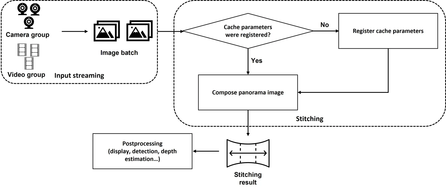
Camera stitching pipeline overview
💡 Rule of thumb: the Field-of-View Intersection-over-Union ratio between each camera pair should be at least 30% to overcome lens distortion and leave enough detectable features for stitching.

Stitching Algorithm

I implemented two stitching algorithms: a simple version with a lighter workflow, and an advanced version that trades higher processing latency for a smoother, more refined result.
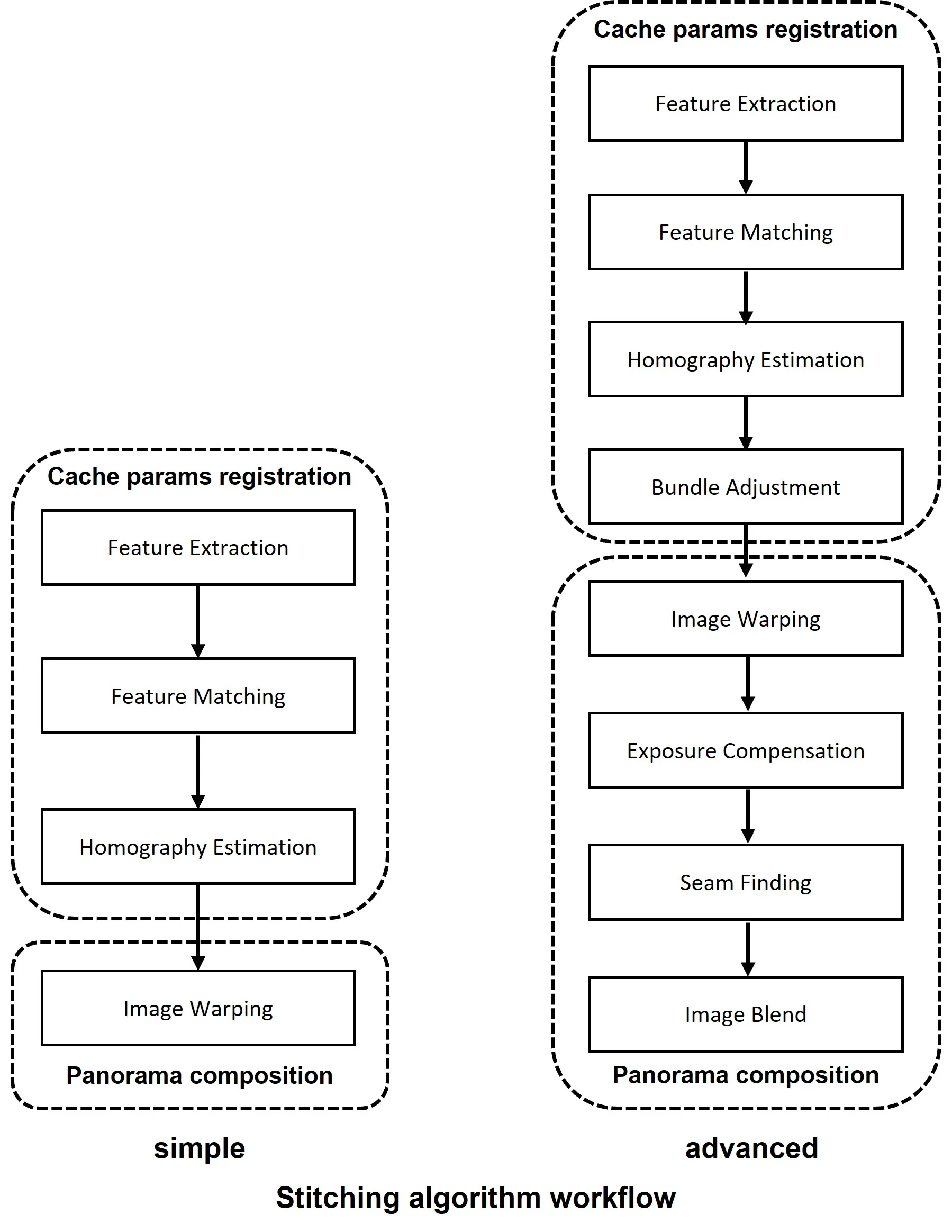
Simple vs advanced stitching algorithm workflow

Feature Extraction

Used to extract the feature list from each input image:

Feature Matching

Used to find matched features between each input pair, from which the homography matrix is estimated:

The homography matrix $H$ defines the transformation between two planes, up to a scale factor:

$$s \begin{bmatrix} x' \\ y' \\ 1 \end{bmatrix} = \mathbf{H} \begin{bmatrix} x \\ y \\ 1 \end{bmatrix} = \begin{bmatrix} h_{11} & h_{12} & h_{13} \\ h_{21} & h_{22} & h_{23} \\ h_{31} & h_{32} & h_{33} \end{bmatrix} \begin{bmatrix} x \\ y \\ 1 \end{bmatrix}$$

$H$ is a $3 \times 3$ matrix with 8 degrees of freedom, since it's estimated only up to scale — typically normalized with $h_{33} = 1$.

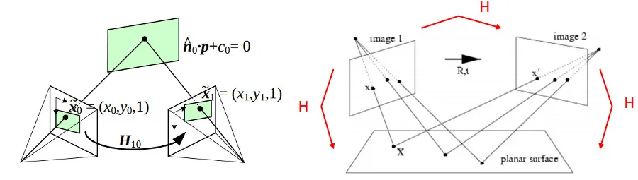
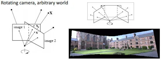
These three cases all relate a transformation between two planes:
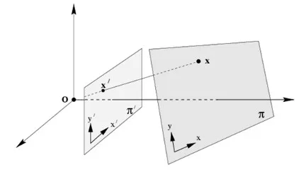
Planar surface and the image plane Planar surface viewed by two camera positions Camera rotating around its axis of projection

Left → right: a planar surface and the image plane; a planar surface viewed by two camera positions (the stitching case); a camera rotating around its axis of projection — equivalent to points lying on a plane at infinity (smartphone panorama mode), the foundational case for image stitching.


Demo

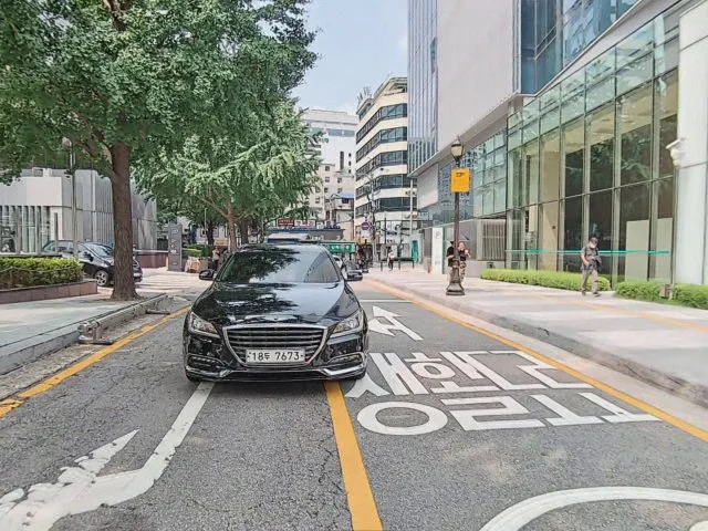
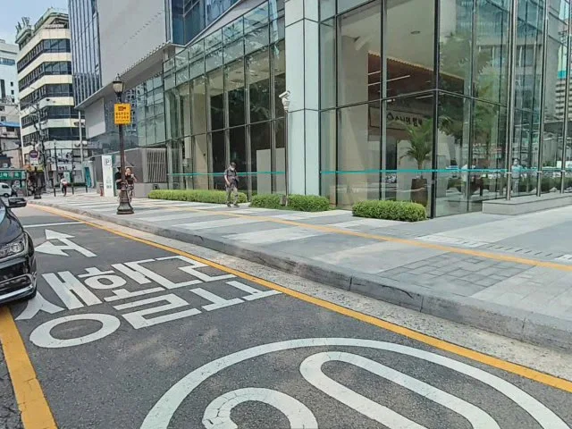
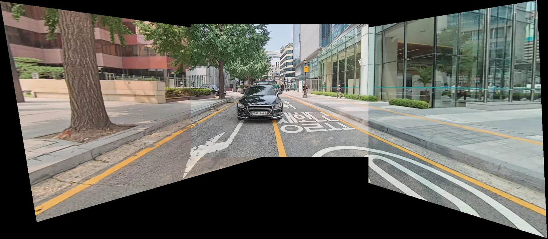
Input — 3 cameras (left mirror, front, right mirror)
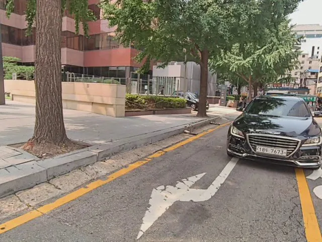
Left mirror camera input Front camera input Right mirror camera input

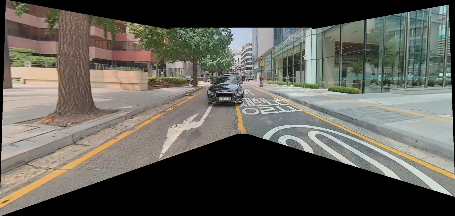
Simple-algorithm output

Simple algorithm stitched output

Advanced-algorithm output
Advanced algorithm stitched output
Depth Estimation

Worker Localization at the Railroad

Introduction

A proof-of-concept to detect and estimate the position of workers at the railroad using a single thermal camera (Boson LWIR).


Process

The pipeline combines two deep learning models: object detection to find the worker, and monocular depth estimation to estimate distance. We picked two SOTA models at the time — YOLOv5 for detection and NeWCRFs for depth — then fine-tuned both on our own data, since the pretrained weights were trained on RGB images and our camera is thermal.

As the first developer on the project, my primary task was sourcing the "depth" ground truth. Given an Ouster OS0 Ultra-Wide High-Resolution Imaging LIDAR, that broke into three sub-tasks:

1. Camera Calibration

Estimating the thermal camera's intrinsic parameters and distortion coefficients via a standard checkerboard-detection approach, based on OpenCV and the ROS image_pipeline/camera_calibration package, plus CLAHE (Contrast Limited Adaptive Histogram Equalization) to sharpen local contrast. Since a thermal camera can't visually distinguish a checkerboard's black and white squares, I held the board under a high-temperature environment (direct sun, halogen light) — black surfaces absorb more heat than white ones, which made the pattern visible to the sensor.

2. Data Collection

Used ROS for synchronized multi-sensor recording: ouster_ros for the LIDAR, flir_boson_usb for the thermal camera, and rosbag record to capture both streams. Synchronization relied on the timestamps ROS attaches at recording time.

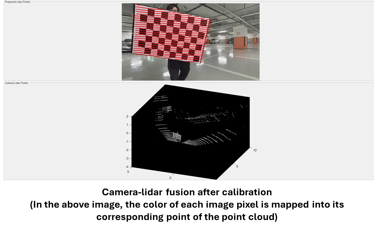
3. Camera-LIDAR Calibration

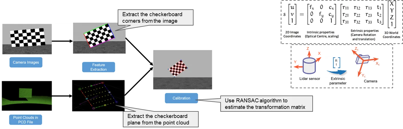
Estimated the rotation matrix and translation vector between the LIDAR and camera coordinate systems:

Camera-LIDAR calibration process diagram 1 Camera-LIDAR calibration process diagram 2

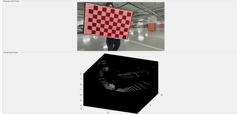
With rotation $R$ and translation $t$, the LIDAR point cloud converts into the camera coordinate system, then projects onto the image plane to form a ground-truth-scale depth map aligned with the camera image:

$$s \begin{bmatrix} u\\ v \end{bmatrix} = \begin{bmatrix} f_x & 0 & c_x \\ 0 & f_y & c_y \\ 0 & 0 & 1 \end{bmatrix} \begin{bmatrix} X_c\\ Y_c \\ Z_c \end{bmatrix}$$
Resulting ground-truth depth map aligned with the thermal camera image

Lesson Learned

This dataset and calibration pipeline helped the team become 1 of 8 solutions worldwide to outperform the provided SOTA baseline on any of the pointcloud- or image-based metrics at the CVPRW 2023 monocular depth estimation challenge. We customized PixelFormer (the SOTA depth model at the time) with training-time augmentations (random crop/rotation, left-right flip, CutDepth) and a zero-padding technique at inference to preserve the training resolution.

Depth Estimation

Real-time PseudoLiDAR

Introduction

An R&D project to replace LIDAR with a camera: an absolute depth estimation model combined with camera calibration parameters generates a pseudo point cloud directly from image pixels, rendered in real time with OpenGL and Open3D.

The underlying theory — human depth perception cues, absolute vs. relative depth estimation, the depth-to-3D-coordinate math, and the proposed multi-camera LIDAR-replication pipeline — is written up separately:


Lightweight Depth Estimation Model

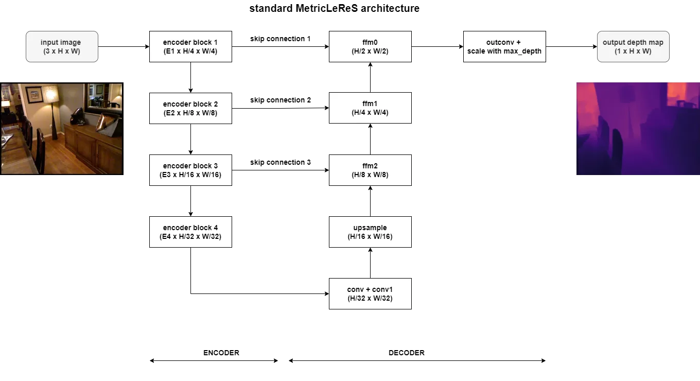
For real-time demonstration, we built an optimized depth model targeting low latency without giving up too much accuracy. Inspired by the YOLO family's efficiency, the model uses a customized YOLOv8 backbone + neck as a 4-scale feature encoder, connected via skip connections to a U-Net-style decoder that reconstructs the depth map.

Lightweight YOLOv8-based encoder-decoder depth model architecture

Fine-tuned on NYUv2 (indoor) and KITTI (outdoor), the model performs competitively against established depth-evaluation metrics while staying far smaller than SOTA methods:

NYUv2 dataset

ModelParamsFPS (480×640)Abs.Rel↓RMSE↓Sqr.Rel↓δ1↑δ2↑δ3↑
Ours (YOLOv8s encoder)10,810,4651050.10330.37170.05780.89650.98140.9958
NeWCRFs270,444,877140.09580.33310.04510.92150.99150.9980
PixelFormer270,895,920160.09050.32420.04350.92890.99060.9977

KITTI dataset

ModelParamsFPS (480×640)Abs.Rel↓RMSE↓Sqr.Rel↓δ1↑δ2↑δ3↑
Ours (YOLOv8s encoder)10,810,4651050.04792.38790.17980.97210.99520.9982
NeWCRFs270,444,877140.05092.18710.16080.97620.99630.9987
PixelFormer270,895,920160.05422.37480.18170.97240.99550.9984

At roughly 7× the FPS of NeWCRFs/PixelFormer and ~4% of their parameter count, the model trades a modest amount of accuracy for the throughput a real-time PseudoLiDAR pipeline needs.

Computer Vision

Head Pose Estimation

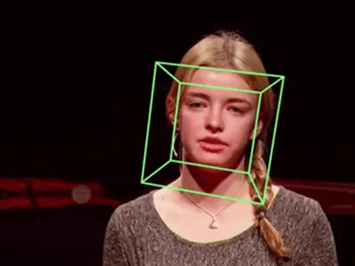
Head pose estimation demo 1 Head pose estimation demo 2

Defining a Head Pose

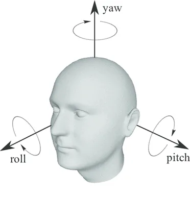
A head pose is defined by a starting point $p = (u_0, v_0)$ — the origin of the head-pose coordinate system — and a rotation matrix (ZYX convention) built from Pitch $Pi$, Yaw $Ya$, and Roll $Ro$:

$$R_z(Ro) = \begin{bmatrix} \cos{Ro} & -\sin{Ro} & 0 \\ \sin{Ro} & \cos{Ro} & 0 \\ 0 & 0 & 1 \end{bmatrix}$$
$$R_y(Ya) = \begin{bmatrix} \cos{Ya} & 0 & \sin{Ya} \\ 0 & 1 & 0 \\ -\sin{Ya} & 0 & \cos{Ya} \end{bmatrix}$$
$$R_x(Pi) = \begin{bmatrix} 1 & 0 & 0 \\ 0 & \cos{Pi} & -\sin{Pi} \\ 0 & \sin{Pi} & \cos{Pi} \end{bmatrix}$$

The combined head-pose rotation matrix with respect to the camera is:

$$R = \begin{bmatrix} \cos{Ro}\cos{Ya} & \cos{Ro}\sin{Ya}\sin{Pi} - \sin{Ro}\cos{Pi} & \cos{Ro}\sin{Ya}\cos{Pi} + \sin{Ro}\sin{Pi} \\ \sin{Ro}\cos{Ya} & \sin{Ro}\sin{Ya}\sin{Pi} + \cos{Ro}\cos{Pi} & \sin{Ro}\sin{Ya}\cos{Pi} - \cos{Ro}\sin{Pi} \\ -\sin{Ya} & \cos{Ya}\sin{Pi} & \cos{Ya}\cos{Pi} \end{bmatrix}$$

Every point $(x, y, z)$ on the head-pose ray follows:

$$\begin{cases} t \geq 0 \\ x = x_0 + t\cos(Ro)\cos(Ya) \\ y = y_0 + t\sin(Ro)\cos(Ya) \\ z = z_0 - t\sin(Ya) \end{cases}$$

Conversely, Pitch, Yaw, and Roll can be recovered from $R$:

$$\tan(Pi) = \frac{R_{2,1}}{R_{2,2}} \qquad \tan(Ya) = -\frac{R_{2,0}}{\sqrt{R_{2,1}^2 + R_{2,2}^2}} \qquad \tan(Ro) = \frac{R_{1,0}}{R_{0,0}}$$

Idea

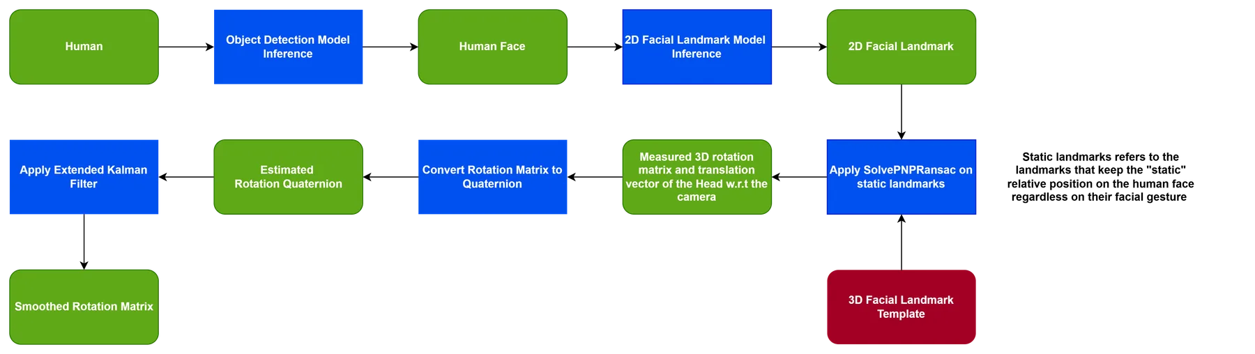
To estimate a human's head pose (rotation matrix + translation vector relative to the camera) in real time, the pipeline follows a classical computer-vision approach:

Head pose estimation pipeline diagram

An Extended Kalman Filter "smooths" the predicted pose and mitigates failures when the model can't see the face — occlusion, extreme angles, etc.


Facial Landmark Estimation

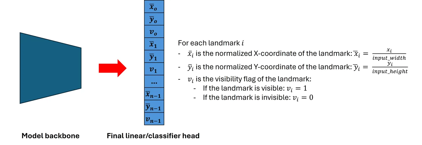
I built a 2D facial landmark model with a classification-style backbone, ending in a linear (classifier) head with $(num\_keypoints \times 3)$ outputs for the with-visibility-flag variant, or $(num\_keypoints \times 2)$ for the without-visibility-flag variant:

Facial landmark model architecture

Head Pose via SolvePnPRansac

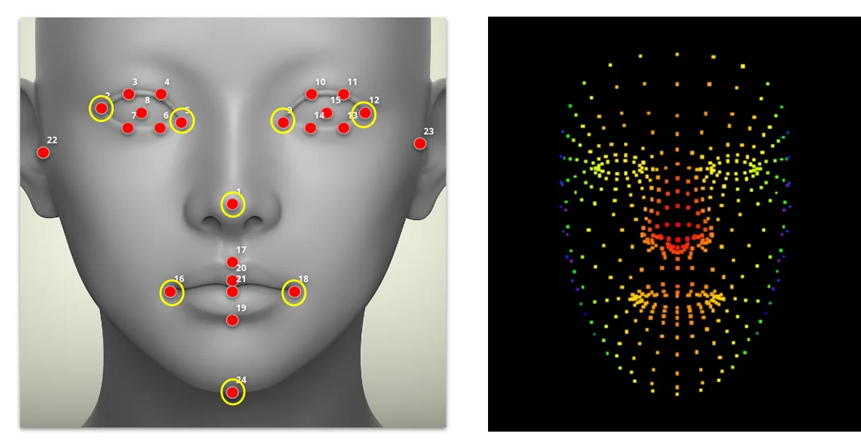
Static points from the predicted 2D landmarks are matched against their corresponding 3D points from the Mediapipe 3D facemark template, then solvePnPRansac recovers the rotation matrix and translation vector. "Static" here means points that keep a fixed relative position to the face even through facial gestures — blinking, yawning, smiling, etc.

2D landmark to 3D facemark template matching

Kalman Filter Stabilizer

The Extended Kalman Filter smooths head-pose motion across frames and bridges gaps when the 2D facial landmark model fails to predict a landmark — most commonly due to occlusion.


References